LLM Deep Dive 3: Rotary Positional Embedding with MiniMind

The previous post tore down classic sinusoidal position encoding: elegant math, but its relative-position rotation property gets shredded once you add embeddings and pass through learned projection matrices. RoPE is the surgical fix: preserve geometric structure directly in the attention space instead of hoping the network rediscovers it.

You can read the original paper summary in my Paper Pulse section. This post is a systems-level reverse engineering: what rotates, why it survives the dot product, how we stretch it past training length, and where people still trip up.

TL;DR

RoPE makes relative distance an intrinsic linear algebra artifact inside the $QK^T$ computation by rotating $q$ and $k$ in paired dimensions using position-dependent angles. After rotation: $(R_m q_m)^T (R_n k_n) = q_m^T R_{n-m} k_n$ ⇒ dependence only on offset $(n-m)$ . That survives projection because the rotation is applied post-projection, not pre.

The key is about rotation

Goal: encode relative distance without an explicit learned bias matrix or extra parameters. Strategy: represent each 2D slice of the projected query/key as a complex number and rotate it by an angle proportional to absolute position. When two positions differ by $\Delta$ , their inner product turns into a relative rotation.

We only touch $Q$ and $K$ (leave $V$ alone). Additive fusion (token + position) is replaced by multiplicative geometric transformation.

Desired behavior of $q_m^T k_n$ after positional injection:

Stable magnitude across large absolute indices.
Systematic phase shift proportional to $(n-m)$ .
No need to reconstruct relative distance through learned weights.

Take two dimensional embedding as an example. Interpret $(x_{2i}, x_{2i+1})$ as $x_{2i} + j x_{2i+1}$ . Rotate by $e^{j m \theta_i}$ . In real block form this is multiplying $q$ at position $m$ with $R_m$ and $k$ at position $n$ with $R_n$ .

R_m q_m = \begin{pmatrix} \cos(m\theta) & -\sin(m\theta) \\ \sin(m\theta) & \cos(m\theta) \end{pmatrix} = \begin{pmatrix} q_{m}^{(0)} \\ q_{m}^{(1)} \end{pmatrix}

R_n k_n = \begin{pmatrix} \cos(n\theta) & -\sin(n\theta) \\ \sin(n\theta) & \cos(n\theta) \end{pmatrix} = \begin{pmatrix} k_{n}^{(0)} \\ k_{n}^{(1)} \end{pmatrix}

Inner product after rotation:

(R_m q_m)^T (R_n k_n)=q_m^T R_m^T R_n k_n = q_m^T R_{n-m} k_n

Since $R_m^T R_n = R_{n-m}$ (orthogonal group property), we have relative-only dependence.

When dealing higher dimension embedding, we simply group the vectors in pairs, with every two dimensions forming a complex number, corresponding to a vector in the complex plane.

\underbrace{ \begin{pmatrix} \cos(m\theta_{0}) & -\sin(m\theta_{0}) & 0 & 0 & \cdots & 0 & 0 \\ \sin(m\theta_{0}) & \cos(m\theta_{0}) & 0 & 0 & \cdots & 0 & 0 \\ 0 & 0 & \cos(m\theta_{1}) & -\sin(m\theta_{1}) & \cdots & 0 & 0 \\ 0 & 0 & \sin(m\theta_{1}) & \cos(m\theta_{1}) & \cdots & 0 & 0 \\ \vdots & \vdots & \vdots & \vdots & \ddots & \vdots & \vdots \\ 0 & 0 & 0 & 0 & \cdots & \cos(m\theta_{\frac{d}{2}-1}) & -\sin(m\theta_{\frac{d}{2}-1}) \\ 0 & 0 & 0 & 0 & \cdots & \sin(m\theta_{\frac{d}{2}-1}) & \cos(m\theta_{\frac{d}{2}-1}) \end{pmatrix}}_{R_m} \begin{pmatrix} q_m^{(0)} \\ q_m^{(1)} \\ q_m^{(2)} \\ q_m^{(3)} \\ \vdots \\ q_m^{(d-2)} \\ q_m^{(d-1)} \end{pmatrix}

Relative structure persists dimension-wise. Frequencies: $\theta_i = 10000^{-2i/d}$ (original RoPE / Sinusoidal style) OR alternative bases (e.g. $10^6$ in many modern LLMs for longer native span). Lower $i$ ⇒ larger $\theta_i$ ⇒ faster phase advance.

Because $R_m$ is block-diagonal with 2×2 rotations, we can implement rotation via element-wise ops + half-swap (no full matmul):

R_m \cdot q_m = \begin{pmatrix}q_m^{(0)}\\q_m^{(1)}\\q_m^{(2)}\\q_m^{(3)}\\\vdots\\q_m^{(d-2)}\\q_m^{(d-1)}\end{pmatrix} \otimes \begin{pmatrix}\cos (m\theta_0)\\\cos (m\theta_0)\\\cos (m\theta_1)\\\cos (m\theta_1)\\\vdots\\\cos (m\theta_{d/2-1})\\\cos (m\theta_{d/2-1})\end{pmatrix} + \begin{pmatrix}-q_m^{(1)}\\q_m^{(0)}\\-q_m^{(3)}\\q_m^{(2)}\\\vdots\\-q_m^{(d-1)}\\q_m^{(d-2)}\end{pmatrix} \otimes \begin{pmatrix}\sin (m\theta_0)\\\sin (m\theta_0)\\\sin (m\theta_1)\\\sin (m\theta_1)\\\vdots\\\sin (m\theta_{d/2-1})\\\sin (m\theta_{d/2-1})\end{pmatrix}

where $\otimes$ is Hadamard product.

Summary Snapshot

RoPE vs Sinusoidal:

Sinusoidal: add position vector before projection → rotation structure lost after $W_Q, W_K$ mixing.
RoPE: rotate $q, k$ post-projection in paired dims → relative offset encoded algebraically in attention scores.

Implementation essentials:

Head dim must be even (pairing).
Rotation angle for pair $i$ : $m\theta_i$ .
$\theta_i$ geometrically decays to expand wavelength range (multi-scale coverage).
Fast to apply: use duplicate cos/sin arrays and half-rotate op (swap + negate second half).

Benefits:

Parameter-free.
Cache-friendly (precompute cos/sin up to max length; slice per batch).
Relative distance naturally emerges; no extra bias tables.
Better length generalization than additive sinusoidal (still not magic beyond trained zone without scaling tricks).

Edge notes:

Still sensitive to extreme lengths; phase wrapping can cause aliasing if base too small.
High-frequency pairs degrade quicker under extrapolation; scaling methods (NTK / YaRN / Dynamic NTK) modulate frequencies.

Extrapolation

Pretraining fixes a max index $L_{train}$ . Beyond that, naive RoPE suffers phase compression and attention destabilization: high-frequency bands wrap multiple times; low-frequency ones are too smooth to differentiate far ranges.

Three families of solutions:

Train longer (brute force): more FLOPs, memory explosion (quadratic attention cost).
Architectural change: sparse / linear / chunked attention (changes model semantics; out-of-scope here).
Frequency scaling hacks (what most production LLMs do): adjust $\theta_i$ mapping so effective wavelengths stretch.

Popular scaling methods:

NTK scaling: non-linear map of position indices before rotation → matches training kernel behavior at longer lengths.
YaRN (used in MiniMind style code below): two-region scaling; preserve low-frequency resolution, compress high-frequency to avoid aliasing.
Dynamic/linear scaling: simple multiply of position index; crude but works for modest extension.

Why scaling works: relative phase progression is slowed so that attention similarity patterns seen during training replay over extended spans without destructive interference.

Failure modes when done wrong:

Over-scaling → loss of local discrimination (everything looks near).
Under-scaling → phase wrap chaos (spurious long-range attention spikes).
Abrupt piecewise transitions → gradient shocks in fine-tuning.

I’ll deep dive comparative scaling math (NTK vs YaRN vs hybrid) in a separate post.

Implementation in MiniMind

The key component of RoPE is implemented at model/model_minimind.py:

1
def precompute_freqs_cis(dim: int, end: int = int(32 * 1024), rope_base: float = 1e6,
2
                         rope_scaling: Optional[dict] = None):
3
    freqs = 1.0 / (rope_base ** (torch.arange(0, dim, 2)[: (dim // 2)].float() / dim))
4
    if rope_scaling is not None:
5
        orig_max, factor, beta_fast, beta_slow = (
6
            rope_scaling.get("original_max_position_embeddings", 2048), rope_scaling.get("factor", 4),
7
            rope_scaling.get("beta_fast", 4.0), rope_scaling.get("beta_slow", 1.0)
8
        )
9
        if end / orig_max > 1.0:
10
            corr_dim = next((i for i in range(dim // 2) if 2 * math.pi / freqs[i] > orig_max), dim // 2)
11
            power = torch.arange(0, dim // 2, device=freqs.device).float() / max(dim // 2 - 1, 1)
12
            beta = beta_slow + (beta_fast - beta_slow) * power
13
            # λ = (β·α - β + 1)/(β·α) YaRN标准公式
14
            scale = torch.where(torch.arange(dim // 2, device=freqs.device) < corr_dim, (beta * factor - beta + 1) / (beta * factor), 1.0 / factor)
15
            freqs = freqs * scale
15 collapsed lines
16

17
    t = torch.arange(end, device=freqs.device)
18
    freqs = torch.outer(t, freqs).float()
19
    freqs_cos = torch.cat([torch.cos(freqs), torch.cos(freqs)], dim=-1)
20
    freqs_sin = torch.cat([torch.sin(freqs), torch.sin(freqs)], dim=-1)
21
    return freqs_cos, freqs_sin
22

23

24
def apply_rotary_pos_emb(q, k, cos, sin, position_ids=None, unsqueeze_dim=1):
25
    def rotate_half(x):
26
        return torch.cat((-x[..., x.shape[-1] // 2:], x[..., : x.shape[-1] // 2]), dim=-1)
27

28
    q_embed = (q * cos.unsqueeze(unsqueeze_dim)) + (rotate_half(q) * sin.unsqueeze(unsqueeze_dim))
29
    k_embed = (k * cos.unsqueeze(unsqueeze_dim)) + (rotate_half(k) * sin.unsqueeze(unsqueeze_dim))
30
    return q_embed, k_embed

Pre-computation of frequency

precompute_freqs_cis builds a reusable cache of $\cos(m\theta_i), \sin(m\theta_i)$ for positions $m \in [0, end)$ . Inputs:

dim: head dimension (per attention head), must be even.
end: max sequence length to cache (not necessarily current batch length; can overshoot for reuse).
rope_base: base for geometric progression; larger base → slower decay of $\theta_i$ → longer native span.
rope_scaling: optional dict enabling length extrapolation (YaRN-style in this code).

Frequency construction

1
freqs = 1.0 / (rope_base ** (torch.arange(0, dim, 2)[: (dim // 2)].float() / dim))

Even indices form $dim/2$ frequency anchors.
Larger index → smaller frequency value → longer wavelength (slower rotation).
Geometric progression: ratio between adjacent pairs = rope_base ** (1/dim).

YaRN scaling (optional)

Activated only if:

1
if rope_scaling is not None and end / orig_max > 1.0:

Steps:

orig_max: original trained max length (e.g. 2048).
factor: target multiple (e.g. 4 → reach 8192).
corr_dim: first frequency whose wavelength (> orig_max) triggers two-phase scaling.
Smooth $\beta$ schedule (slow → fast) across dims:

1
power = torch.arange(0, dim//2)/ (dim//2 - 1)
2
beta = beta_slow + (beta_fast - beta_slow) * power

YaRN scale per dim:

1
scale = ((beta * factor - beta + 1)/(beta * factor))    # for dims < corr_dim
2
scale = 1/factor                                        # for dims ≥ corr_dim

Effect: retain discriminative low-frequency rotation granularity while damping high-frequency wrap risk.
Apply: freqs *= scale.

Expand over positions

1
t = torch.arange(end)
2
angles = torch.outer(t, freqs)  # shape: (end, dim/2)

Cache cos/sin

1
freqs_cos = cat([cos(angles), cos(angles)], -1)
2
freqs_sin = cat([sin(angles), sin(angles)], -1)

Duplication restores full head_dim (each pair uses (x_even, x_odd)).

Returned: (freqs_cos, freqs_sin) of shape (end, dim).

Visual intuition

Two-region scaling: left region (lower dims) gets gentle wavelength stretch; right region (higher dims) gets uniform compression → mitigates aliasing. Diagram:

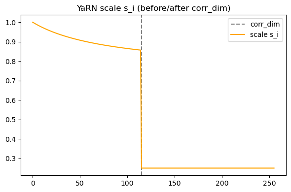
Rule of thumb: confirm no dimension’s effective wavelength collapses below typical phrase length, and no high-frequency pair wraps > ~8× within target window.

Wrap up

RoPE is a geometry-preserving positional system: cheap, deterministic, and extensible with scaling tricks. It converts “where” into controlled phase shifts instead of injected additive noise.