LLM Deep Dive 4: Normalization (LayerNorm vs RMSNorm) in MiniMind

Why normalization is needed

Deep transformers stack dozens to hundreds of residual blocks. Without normalization, signal statistics (mean/variance/scale) drift layer by layer—making gradients chaotic and learning rate tuning a nightmare.

Classic explanation: reduce “internal covariate shift” (distribution drift between layers). Modern practical view: keep feature scales bounded so residual paths remain numerically sane, enabling:

Stable gradient propagation (avoid exploding/vanishing)
Higher usable learning rates (especially with AdamW + warmup)
Reduced sensitivity to weight init
Cleaner residual “identity highways” in pre-norm architectures

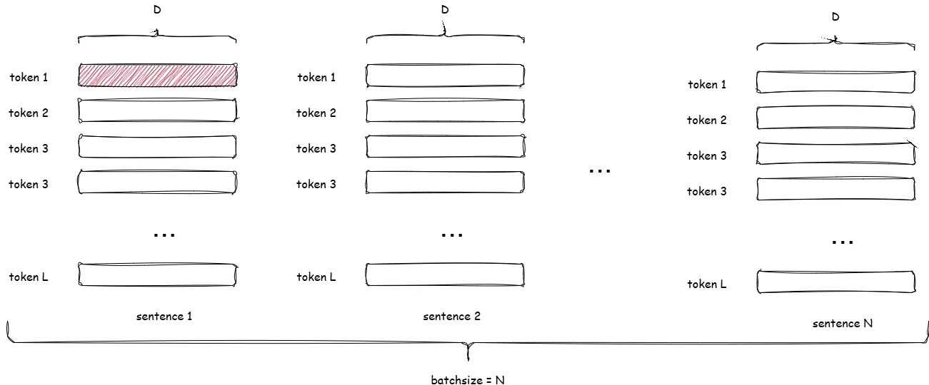
Think of normalization as inserting a cheap re-centering/re-scaling checkpoint that bounds error amplification. In transformers we normalize per-token over hidden dimension, NOT across batch, so inference is invariant to batch size.

LayerNorm & RMSNorm

In transformer-style LLMs the two players are LayerNorm (canonical) and RMSNorm (leaner). Both operate per token vector (last dimension only). No batch coupling.

LayerNorm

Let input tensor shape be $(N, L, D)$ = (batch, sequence length, hidden size). LayerNorm acts independently on each token vector of length $D$ .

For token at batch index $n$ , position $l$ , denote its vector $x_{n,l} \in \mathbb{R}^D$ . Compute:

\mu_{n,l} = \frac{1}{D}\sum_{i=1}^D x_{n,l}^{(i)}

\sigma_{n,l}^2 = \frac{1}{D}\sum_{i=1}^D\big(x_{n,l}^{(i)}-\mu_{n,l}\big)^2

Then

\hat{x}_{n,l}^{(i)} = \frac{x_{n,l}^{(i)} - \mu_{n,l}}{\sqrt{\sigma_{n,l}^2 + \epsilon}}

Affine restore step (learnable scale/shift per feature):

y_{n,l}^{(i)} = \gamma_i\,\hat{x}_{n,l}^{(i)} + \beta_i

Why keep $(\gamma, \beta)$ ? Normalization scrubs amplitude & offset; these params let the model reintroduce optimal feature scaling for downstream layers. Without them capacity collapses subtly.

Operational notes:

Independent of batch size and sequence length.
Stable under mixed precision; $\epsilon$ (often 1e-5 or 1e-6) guards underflow.
Cost: mean + variance reduction + two passes; slightly heavier than RMSNorm.

RMSNorm

MiniMind swaps LayerNorm for RMSNorm: drop mean centering; scale only by root-mean-square. Leaner, fewer ops, empirically fine for modern LLM residual stacks.

Definition for vector $x \in \mathbb{R}^D$ :

\text{RMS}(x) = \sqrt{\frac{1}{D}\sum_{i=1}^D x_i^2 + \epsilon}

\text{RMSNorm}(x) = \gamma \cdot \frac{x}{\text{RMS}(x)}

No $\beta$ shift; mean is preserved (not forced to 0).

Tradeoffs vs LayerNorm:

Pros: Fewer reductions (no mean separate + variance), faster, less numerical churn.
Cons: Does not center -> downstream layers must tolerate mean drift (residual pathways usually do).
Behavior: Invariant to uniform scaling (like LayerNorm), not invariant to constant bias.

Implementation of RMSNorm in MiniMind

Straightforward module:

1
class RMSNorm(torch.nn.Module):
2
    def __init__(self, dim: int, eps: float = 1e-5):
3
        super().__init__()
4
        self.eps = eps
5
        self.weight = nn.Parameter(torch.ones(dim))
6

7
    def _norm(self, x):
8
        return x * torch.rsqrt(x.pow(2).mean(-1, keepdim=True) + self.eps)
9

10
    def forward(self, x):
11
        return self.weight * self._norm(x.float()).type_as(x)

Key mechanics:

Scale factor: rsqrt(mean(x^2) + eps).
Keeps mean; only shrinks/expands magnitude.
Single parameter weight (i.e. $\gamma$ ) per feature.
Cast to float improves stability under bf16/FP16.
Works per token: shape broadcast (N,L,D) over last dim.

Pre-Norm vs Post-Norm

Where do we apply norm in a residual block?

Post-norm (old Transformer 2017):

1
x -> Attention(x) -> + x -> LayerNorm -> out

Gradient must traverse the normalization that sees the sum; variance drift across deep stacks perturbs its scale factor — hazard for very deep (>24L) models.

Pre-norm (modern LLMs):

1
x -> LayerNorm(x) -> Attention -> + x -> out

Now backprop has an always-present identity shortcut: derivative includes a clean +1 term independent of attention internals. That stabilizes gradients; norms do not collapse/explode as depth grows.

Intuition (hack-level): keep raw residual untouched until after the heavy op; you guarantee a loss gradient highway unblocked by adaptive statistics. Empirically speeds convergence, removes the need for crazy warmup schedules, and helps with larger learning rates.

MiniMind uses pre-norm for both attention and MLP sublayers.

Implementation excerpts (trimmed):

1
class MiniMindBlock(nn.Module):
2
    def __init__(...):
3
        self.input_layernorm = RMSNorm(config.hidden_size, eps=config.rms_norm_eps)
4
        self.post_attention_layernorm = RMSNorm(config.hidden_size, eps=config.rms_norm_eps)
5

6
    def forward(...):
7
        residual = hidden_states
8
        hidden_states, present_key_value = self.self_attn(
9
            self.input_layernorm(hidden_states),  # pre-attention RMSNorm
10
            position_embeddings, ...
11
        )
12
        hidden_states += residual
13
        hidden_states = hidden_states + self.mlp(self.post_attention_layernorm(hidden_states))  # pre-MLP RMSNorm
14

15
class MiniMindModel(nn.Module):
6 collapsed lines
16
    def __init__(...):
17
        self.norm = RMSNorm(config.hidden_size, eps=config.rms_norm_eps)
18

19
    def forward(...):
20
        ...
21
        hidden_states = self.norm(hidden_states)  # final RMSNorm

BatchNorm (side note)

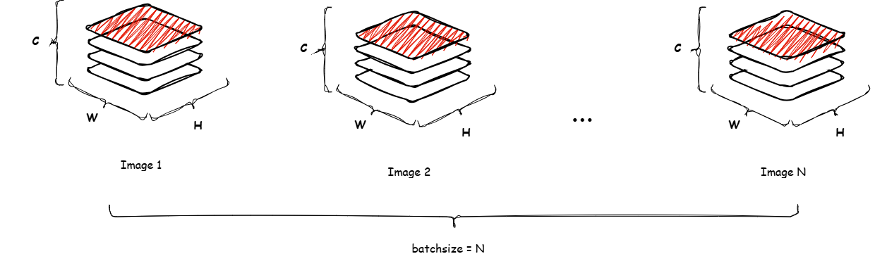
BatchNorm normalizes per-channel over the mini-batch (and spatial dims for CNNs). Rare in autoregressive LLMs because batch-size dependence breaks variable-batch inference stability and hurts long-context streaming.

Shape $(N,C,H,W)$ :

Per-channel mean:

\mu_c = \frac{1}{N H W}\sum_{n,h,w} x_{n,c,h,w}

Per-channel variance:

\sigma_c^2 = \frac{1}{N H W}\sum_{n,h,w} (x_{n,c,h,w}-\mu_c)^2

Normalize:

\hat{x}_{n,c,h,w} = \frac{x_{n,c,h,w}-\mu_c}{\sqrt{\sigma_c^2+\epsilon}}

Affine:

y_{n,c,h,w} = \gamma_c \hat{x}_{n,c,h,w} + \beta_c

Running (EMA) stats updated during training (momentum $m$ ):

\tilde{\mu}_c \leftarrow m\tilde{\mu}_c + (1-m)\mu_c

\tilde{\sigma}_c^2 \leftarrow m\tilde{\sigma}_c^2 + (1-m)\sigma_c^2

Inference uses frozen stats:

y = \gamma_c \frac{x-\tilde{\mu}_c}{\sqrt{\tilde{\sigma}_c^2+\epsilon}} + \beta_c

Why not in LLMs: batch-coupling + sequential generation mismatch + extra state sync for distributed training.

Summary

Key takeaways:

LayerNorm: centers + scales per token; heavier; widely used historically.
RMSNorm: scale-only; cheaper; works great with residual pre-norm stacks (MiniMind choice).
Pre-norm blocks preserve an identity gradient path → deeper stable training & higher LR headroom.
BatchNorm: powerful in vision; avoided in autoregressive transformers due to batch dependence.

Rules of thumb:

If reproducing classic papers: LayerNorm is fine.
If chasing speed/memory with similar convergence: pick RMSNorm.
Go pre-norm unless you have shallow depth (<12) and legacy compatibility constraints.